MLB 6. lecture - Naive Bayes + Support Vector Machines + Random Trees

• what is Naive Bayes? It’s a probabilistic classifier based on the Bayes’ Theorem
• why is it naive? Because it makes strong (and often unrealistic) assumption the all features are conditionally independent of each other (given the class label $c$)
  • and it suprisingly works really well
  • when the features are highly correlated, it may overestimate the class probabilities
• based on joint probability (conditional independence), just a reminder:
  • $P(AB)=P(A)\ast P(A|B)=P(B)\ast P(B|A)$
  • $P(AB)=P(A)\ast P(B)$ if $A$ and $B$ are independent
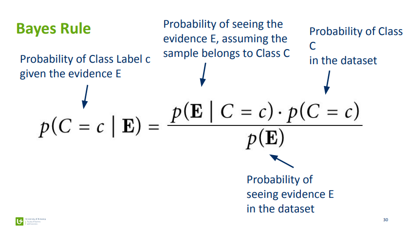
• The main formula:
  • word interpretation:
    • the goal of Naive Bayes is to get probabilities of all available class labels given the current set of features $E$ and then finally predict the class label with the highest probability
      • example: if we got 2 target labels ($c_1$ = Spam, $c_2$ = Not spam), we calculate the probabilities for the currently given features $E$ for both labels and then take the one with higher probability
      • the $p(E)$ in both calculations is the same, we can exclude it and simplify the calculations
    • different wording: for prediction, I have got the given feature set $E$, but not the $c$ label (we need to predict it), so the Naive Bayes will calculate the probability of all labels in the $C$ target feature if this feature set/condition/evidence holds
  • how do we get $p(E|C=c)$?
    • Naive Bayes makes the assumption that the evidence/features are independent of each other given class label $c$
    • $p(E|C=c)=p(e^1|c)\ast p(e^2|c)\ast ...\ast p(e^k|c)$
      • we can just calculate the probability of each feature given the class $c$ (during training) and store it
• advantages:
  • very simple + performs well
    • it does not care about the exact probabilities of the class labels, it just picks the one with the highest probability
  • efficient storage and efficient computation time
    • during training it needs to compute and store $p(E|C)$ values
      • number of features * number of target label classes
      • it’s a probability for the whole feature
      • it does not have to store the values per row and that’s why it’s so efficient
    • and also the $p(C)$ = number of class labels
      • for each value just calculate the number of occurences / all rows count
  • can learn incrementally
• disadvantages
  • as it assumes the conditional independence - it may overestimate class probabilities

Evidence lift framework

• it’s a different way of looking at Naive Bayes (but is not official Naive Bayes), which does not consider the conditional independence, but a multiplicative factors (lifts) for each feature/evidence part
• it takes the standard probability of the target class label, e.g. $p(EmailStatus=Spam)$ and then multiplies it by lifts of each feature/evidence part
  • p(Spam | evidence) = P(Spam) × Lift(e₁) × Lift(e₂) × Lift(e₃) × …
  • example of the feature lift: Lift(HasAds=Yes) = P(HasAds=Yes | Spam) / P(HasAds=Yes) = 5
    • meaning, if the email contains spams, it increases the probability of p(Spam | evidence) with a factor of 5 (multiply by 5)
    • the lift can also be less than 1, for example a lift of 0.01 (if the email contains the work “meeting”)

Support Vector Machines

The problem with linear classificators

• what basically the linear classificators do is learning, where to draw an ideal line (or hyperplane) to distinguish between two classes
  • the line is called a “decision boundary”
  • if it’s possible to draw a line (hyperplane) to separate the two classes perfectly, the dataset is “linearly separable”
    • but this is often not the case in real-world datasets
    • the linear classificators can still perform well, but they will make some misclassification errors
  • each algorithm copes with the optimal decision boundary by itself (using the loss function)

What is Support Vector Machine?

• SVM is a maximum-margin classifier, it determines its decision boundary by maximizing the distance between the optimal boundary and the closest data point from each class
  • these closest data points are called “support vectors” (because they support the optimal decision boundary)
• why are they good / better than other linear classifiers?
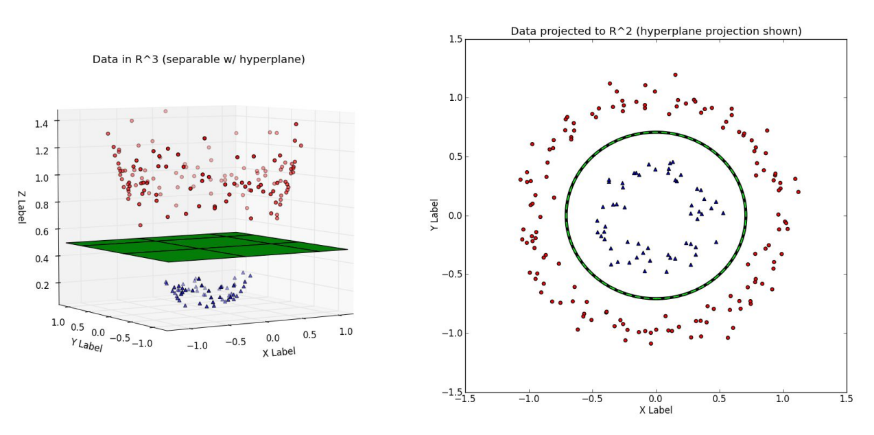
  • because we can use a so called “the kernel trick” to deal even with linearly inseperate data, so the data, where we cannot simply draw a line/hyperplane to separate the data
    • the trick is about projecting the data to a higher dimension feature space, where it’s possible to linearly separate the data
    • the separation is done using the kernel function (linear kernel, polynomial kernel, radial basis function kernel…)
  • 

Random Forests

• a classifier technique based on ensembling (= combining more models to have more accurate predictions than just from the single model), the idea of wisdom of the crowd
• Random Forest is an ensemble of decision trees, which predictions are combined and used as final predictions
  • bagging = each tree is trained on random subset of the data
    • bagging = bootstrap aggregating
    • the data instance is sampled from the dataset and then returned to the original data pool, so it could be sampled again for the same tree
    • then all results are aggregated to get final predictions (average or majority vote is used)
    • the idea is to create an ensemble of weak learners of the same model type (e.g. trees), but it’s possible to create bagging ensembles with diverse models (linear regression, decision trees, neural nets etc.)
  • attribute sampling = each tree uses a random subset of features
    • every node in each tree have a different subset of features
    • the trees are then very diverse, but that’s what we want to have low variance
• the problem of individual Decision trees is easy overfitting (= high variance of the model)
  • the Random Forest can significantly decrease the variance while keeping low bias
• disadvantage = low interpretability, it can consist of hundreds of trees