MLB 3., 4. and 5. lecture - Classification

• supervised learning (meaning that we have labelled data to train on)
  • those training data are “supervising” the training process
• fitting the model = learning which values of features correlate with the label we want to predict (in the training set) and how
  • we need to identify good features (that are useful)
• we also introduce the parametric learning
  • = assigning each feature a weight - by how much it contributes to the output label value
  • predicting the label as the mathematical function of the features * weight
• Machine learning - různá témata (FIT)

Glossary

• sample/instance = row in the table containing all features
• label = target feature that we are trying to classify

Supervised segmentation

• process of separating/splitting the dataset into subgroups
  • we have to find a feature, which best segments the dataset - to create more homogeneous and pure segments with respect to the target variable
    • it is pure, when the segment clearly points to some target variable value
  • we will separate instances into subgroups according to this chosen feature
    • we want those features, which are able to reduce the impurity of the resulting segment
• this is the principle of decision trees
• we usually choose subgroups in subgroups

Decision trees

• Rozhodovací stromy
• tree is created by finding the most informative variable (=feature) which splits the dataset into “pure” subgroups
  • and those subgroups are then splitted into next subgroups according to next most informative variable
  • and this process is repeated until we’re satisfied (or we cannot continue)

Splitting rule

• calculating all possible splits (for all features)
• calculate the goodness of the split
  • GINI index
  • Information gain (derived from Entropy)
• choose the best split (maximizing the purity)

Entropy

• measuring the level of impurity (uncertainty) of the subgroup with respect to the label
• between 0 and 1
• $\sum p_i\ast log(p_i)$
  • $p_1$ - proportion of label 1
  • $p_2$ - proportion of label 2 etc.
  • if $p_1$ = 0.5 and $p_2$ = 0.5, the entropy is 1, meaning the highest level of impurity/uncertainty

Information gain

• = measures the change in the entropy between the parent and child nodes
  • in other words, how much information we gain by splitting the parent into child nodes
  • weight of each child is proportional to the number of instances in this child
  • $IG(parent,children)=entropy(parent)-[p(c_1)\ast entropy(c_1)+p(c_2)\ast entropy(c_2)]$
    • the entropy of each child is weighted by the proportion of entropy of instances belonging to the child
      • the split does not have to be of equal lenghts (one child can get more instances, therefore its information gain has to be scaled proportionally)
• by splitting, we want to maximize the information gain

GINI impurity

• alternative to entropy
  • it is computationally cheaper
• best split minimizes the weighted average GINI impurity
• between 0 and 0.5
• $GINI(node)=1-{\sum }_{i=1}^N{p}_i^2$
• $GINI(split)=p(c_1)\ast GINI(c_1)+p(c_2)\ast GINI(c_2)$
  • the goal is to minimize this weighted split GINI impurity

Stopping rule

• determines, when to stop the recursive splitting the tree in the subgroups
• more rules apply:
  • maximum depth reached
    • prevention from overfitting (and better interpretability)
  • minimum samples per node
    • so the reliable assignment can be made (and it also reduces overfitting)
  • minimum impurity decrease
    • any next split won’t pass the defined purity decrease
    • also helps with the overfitting
• smaller tree = not likely to be overfitted, faster to train, more interpretable

Assignment rule

• determines, which label value is assigned to defined leaf node
• common assignment is to assign the most frequent class present in the node
  • but not in all cases!

Logistic regression

Parametric learning

• trying to predict the label as the mathematical function of the other features (with weights)
  • we have linear, polynomial, linear with feature interactions or neural networks
• model learning is how much each feature contributes to the target label
  • through minimizing the loss function, which measures the error of the predicted values (compared to real target label values)
  • e.g. MSE (mean squared error is used) - see Evaluace
• gradient descent - algorithm for iterative updating the feature weights (=parameters) to minimize the loss function
  • it uses the gradient (= first derivative of the loss function) with respect to the parameters

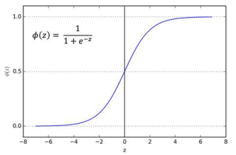
Logistic function

• also known as the sigmoid function - it maps all real numbers to the range [0,1]
• 
• decision boundary is z=0
  • near z=0, small changes near the decision boundary result in big changes in the probability

Logistic regression

• classification algorithm that models the probability of the binary outcome using the Logistic function applied to a linear combination of features (with weights)
• process:
  • we calculate a weighted sum of features (just like linear regression)
    • the result z can be in [-inf, inf]
  • apply the sigmoid function (the logistic function)
    • σ(z) = 1 / (1 + e^(-z))
  • this gives us a P(y=1|x), a probability that the target label is 1 given features $x$
    • if it is more than 0.5, predict 1, othewise predict 0
• output is a probability between 0 and 1 (e.g. there is a 45 % probability that this client will churn this month)
• this is often a baseline classification model and is very interpretable (we instantly know, how much each feature affects the result)
• to transform the probability of the binary result, we apply a decision threshold (it is often 0.5, but now always)

Binary Cross-Entropy

• = a loss function used to learn a logistic regression model
• it measures how far the predicted probabilities are from the actual labels
  • $BCE=-[yᐧlog(\hat{y})+(1-y)ᐧlog(1-\hat{y})]$
  • it has two parts and only one is “activated” based on whether we are testing how far is the prediction from y=0 or y=1
• it penalizes being confidently wrong

How to spot overfitting?

• as high accuracy/low error on the training set and low accuracy/high error on unseen data
• the model has learned a lot of signal (= data useful for generalization) and also a lot of noise (= data that does not lead to generalization)

How to spot underfitting?

• on a learning curve:
  • the training and validation loss are both decreasing (we need more epochs for it to decrease more and see where is the sweet spot (where the loss is minimized))
  • or when the training and validation curve is not decreasing (or just really slowly) ⇒ our model is too simple for the data

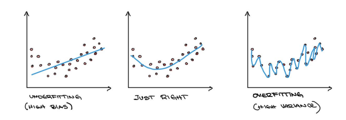
Bias-variance trade-off

• trade off between underfitting and overfitting
• 
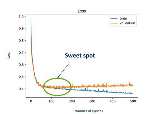
• sweet spot on the learning curve:
  • 
    • when both the training and validation loss is decreasing together
    • and stop at the point, when by more epochs we don’t gain any more loss decrease from the validation “unseen” data

Early stopping

• a technique that prevents both underfitting and overfitting by “watching” the loss on the validation data
  • when the loss on validation data stops decreasing or even start increasing, the technique stops the training and returns the best model (= best weights) found

Regularization

• techniques that penalize the complexity of the model (which prevents overfitting)
  • it prevents the model from learning from the noise in the data (from using too complex patterns)
• L1-regularization (Lasso)
  • adds a sum of current absolute weights multiplied by some $\lambda$ parameter as a penalty
• L2-regularization (Ridge)
  • the same, but instead of absolute weights, use squared weights
• Elastic net (combines L1 and L2)