MLB 5. lecture - How to choose the best model a visualize it's performance

• MLB 3., 4. and 5. lecture - Classification (classification models) have binary outputs (positives = 1 and negatives = 0)
  • positives imply something interesting/alarming
  • negatives are not interesting cases
  • dataset will often be imbalanced (0 > 1)

Accuracy

• (number of correct predictions) / (number of all samples)
• it does not care about the cost of the correct prediction (it is not sufficient by itself)
  • if the dataset is imbalanced with 96 % negatives and the classifier predicts negative 100 % of the time → it still has 96 % accuracy…

Confusion matrix

• complete information: Confusion matrix
• related matrix is: Cost-benefit matrix
  • according to the desired usage of the model, we define:
    • costs for false prediction
      • costs for FP and FN can differ
    • benefit for true prediction
      • benefit = value - cost (beware of the double counting)
      • benefits for TP and TN can differ
  • it’s totally different for different domains (for ads cost/benefits or ordering medical test)
  • using this matrix we can calculate the Expected profit
    • Expected Profit = p(TP)*benefit(TP) + p(TN)*benefit(TN) + p(FP)*cost(FP) + p(FN)*cost(FN)
    • p(X) means the probability of X

Baseline

• a simple model or strategy to which we can compare other models or approaches
  • it should tell us to invest more (or not)
• the usage of concrete baseline differs by the desired usage
• baselines:
  • random classifier = assigns a random label to every sample
    • comparing to this classifier we measure how much did the model learn from the data
    • if the model has the same or similar accuracy, the model learned nothing (it acts as a random classifier)
  • majority classifier = assigns only one label to every sample (the one that is majority, often it is 0)
    • so if the majority of target label is 0, it will without exception assign 0 to all predictions
    • if majority classifier has accuracy 97 % (because the 97 % of all samples are negative), having model accuracy 97.1 % is not that great
  • single data source classifier = uses only one data source
    • we can measure if adding a new data source improves the model or not
  • simple model (logistic regression, decision tree)
    • if we should invest in an advanced modelling techniques or not

Visualizing the performance

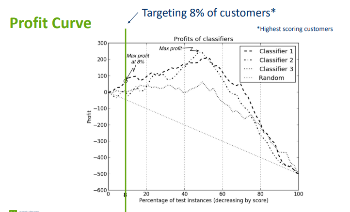
Profit curve

• 
• we score the customers using our classifier (e.g. the higher score means more probability that the customer will buy/convert)
• and the goal is to calculate the profit of targeting top X% of customers
  • it’s the revenue if the customer buys - costs for the targeting (e.g. marketing)
• if we target 0 % of customers, the revenue will be zero (logically)
• if we target 100 %, we will have negative revenue (the cost of targeting is higher than the cost of buys from the best customers) + we don’t need to model
  • the added value of the model is the area between random classifier and the profit curve

ROC curve

• ROC křivka

Cumulative Response Curve

• “How many of the true positives am I reaching if I target X% of the population?”
• for example, if I decide to target 20 % of the population, I get 50 % of the true positives (which is better than random classifier)
• but the information about the false positive rate is missing
  • this chart can be used if the FPS is uniform or the cost of FP is small (e.g. sending an e-mail is cheap)

Lift curve

• is derived from the Cumulative Response Curve
• it just shows the difference between the model probabilities versus the random classifier